Source: 📖 Problem Solving with Algorithms and Data Structures using Python ch8.18

---

What is a strongly connected component?

A strongly connected component \(C\) is a subset of a graph \(G\) (\(C \subset G\)) whose constituent vertices have very strong connections. We can tightly define a strongly connected component as the largest subset of vertices in \(V\) (the set of all vertices in \(G\)) where, for any pair of vertices \(v1, v2 \in C\), a path exists from \(v1\) to \(v2\) and also from \(v2\) to \(v1\). Notice that a path must exist, not an edge (a path can be made up of multiple edges).

In simple terms, any pair of vertices within a strongly connected component (a subset of a graph) must have a path the leads from \(v1\) to \(v2\) and from \(v2\) to \(v1\). The path does not need to be the same path in reverse order, you must simply be able to get from one vertex to the other by following any path.

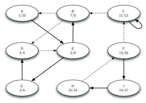
The diagram below illustrates a graph with three strongly connected components, each represented by shaded boundaries.

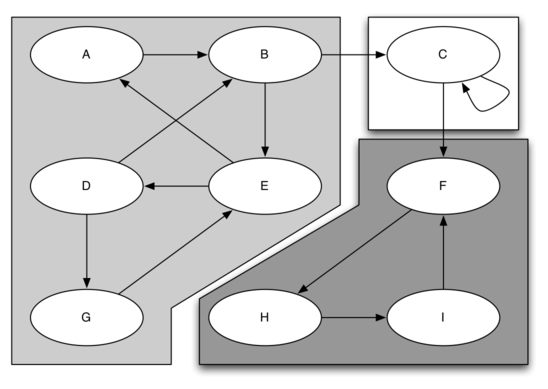
Take the left SCC as an example. If we pick two random vertices, say \(A\) and \(G\), we can follow a path from one to the other in either direction – \(\{A, B, E, D, G\}\) and \(\{G, E, A\}\). This kind of relationship exists between any two vertices within a strongly connected component.

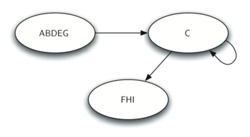
With the strongly connected components of a graph identified, an abstracted, reduced version of the graph can be considered like so:

The implementation of the SCC has four steps:

1. Execute a depth first search on the graph to compute the finish times for each vertex.
2. Compute the transposition of the graph.
3. Execute a depth first search on the transposed graph, visiting each vertex in descending finish time order within the main DFS loop.
4. Each tree in the resulting depth first forest returned in step 3 is a strongly connected component. Output the vertex names/IDs/keys for each tree to identify the components.

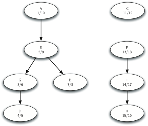
The following image shows the discovery and finish times for each vertex in the graph above after DFS has been executed on the graph.

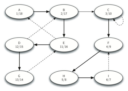
Next we run DFS on the transposed graph, this is the result:

Finally, we output the vertex keys for each tree constructed by the DFS in the previous step.