Source: 📖 Problem Solving with Algorithms and Data Structures using Python 8.22

---

Prim's algorithm

Prim's algorithm is a greedy algorithm which is somewhat similar to Dijkstra's algorithm. They both traverse graphs using breadth first search to return a path through the graph, but their output goals differ in that Dijkstra's aims to return the shortest distance from a starting vertex to any other connected vertex in the graph, whereas Prim's aims to return a minimum weight spanning tree of the graph.

To construct a spanning tree \(T\), Prim's algorithm uses the following methodology:

while T is not yet a spanning tree:
	find an edge that is safe to add to the tree
	add the new edge to T

The important part of this process is the second line, which aims to find a safe edge to add to the spanning tree. A safe edge is defined as an edge that connects a vertex that is already in the spanning tree to a vertex that currently isn't – we don't want multiple edges leading to the same vertex in the output tree as this only adds to the total weight of the tree, so any new edges we add must lead to new vertices. This process also ensures that the output structure remains a tree, which is inherently acyclic.

The python code to implement Prim's algorithm is as follows:

def prim(graph, start):
	pq = PriorityQueue()
	for vx in graph:
		vx.distance = sys.maxint
		vx.predecessor = None
	start.distance = 0
	pq.heapify([(vx.distance, vx) for vx in graph])
	while pq.size > 0:
		current_vx = pq.extract_min()
		for neighbour in current_vx.get_connectons():
			new_cost = current_vx.distance + current_vx.get_weight(neighbour)
			if neighbour in pq and new_cost < neighbour.distance:
				neighbour.predecessor = current_vx
				neighbour.distance = new_cost
				pq.change_priority(neighbour, new_cost)

Like Dijkstra's, Prim's algorithm utilises a priority queue to track which vertices it has yet to visit and in what order to visit them. After initiating the priority queue, we loop through hall the vertices in graph and reset their distance and predecessor attributes to infinity and None respectively. Next, we mark the distance of the starting vertex as 0 before constructing a priority queue out of all the vertices in graph, using the distance as the priority key. This is where the while loop described above begins. In code, we can identify when the spanning tree is complete because every vertex has been visited and connected – this is why the while loop checks to see if there are still any vertices present in the priority queue, because with each pass of the loop we will remove one fully explored vertex.

Inside the loop, the first step is to select a vertex to work on. We select the vertex at the front of the priority queue – that is, the vertex with the smallest distance that has not yet been extracted from the queue. Next we loop through its neighbouring vertices and calculate the distance from the starting vertex to the neighbouring vertex if we were to go through the current vertex being explored. This is the point where Prim's algorithm differs from Dijkstra's – if the new cost is less than the neighbouring vertex's current distance value and if the neighbouring vertex still exists within the priority queue (meaning that it has not yet been added to the spanning tree), then we overwrite its predecessor and distance attributes before changing its priority in the priority queue to reflect these changes.

The process is illustrated below on an example graph:

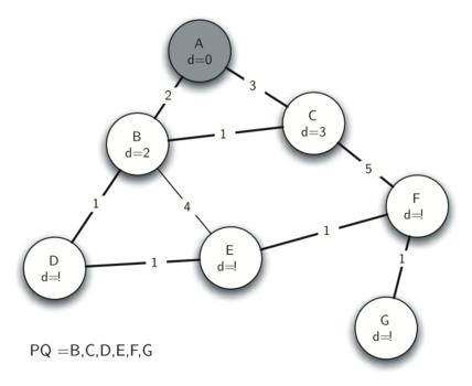
Starting at A, its distance is set to 0, its neighbouring vertices are visited and their distances marked.

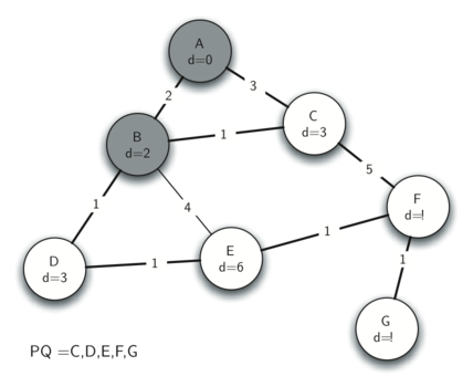
With A explored, the next-closest vertex is B with a distance of 2. All of B's neighbours are visited and their distances updated, only if they still remain in the priority queue and the newly calculated distance is a cost improvement on the existing value. This means that the distance and predecessor of A cannot be updated, as it is no longer part of the priority queue (meaning that it already exists in the output spanning tree). In this example, the distance and predecessor of vertices D and E are updated as they were previously unseen by the algorithm.

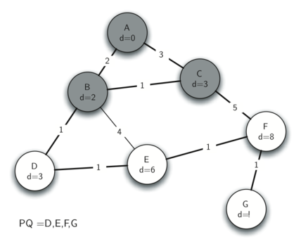
With B's neighbours exhausted, the next-closest vertex is C. C's only unseen neighbour is F, as B is already part of the spanning tree being built. F's distance and predecessor are updated.

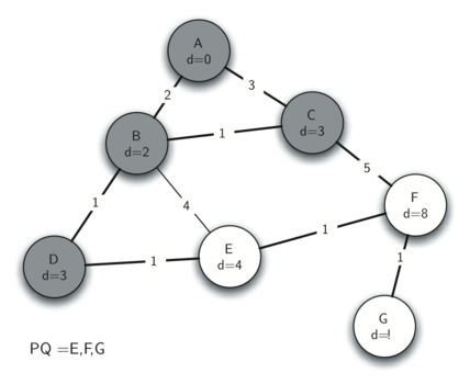
The next-closest vertex is D. D cannot update B's distance as doing so would not be an improvement and B is already part of the spanning tree so it's out of consideration anyway. The path to E, however, can be improved by going through D. E's attributes are updated accordingly, and vertex D, now fully explored, is removed from the priority queue and therefore considered part of the output spanning tree.

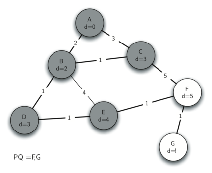
With a distance of 4, E is the next-closest vertex. When exploring E's neighbours, the algorithm identifies that the path to F which is not yet fully explored can be improved by going through E, so F is updated accordingly.

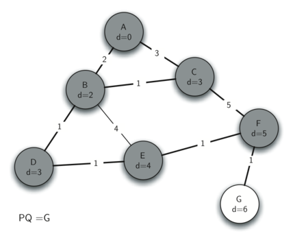
The next-closest vertex is F, as G currently remains unseen by the algorithm. Upon exploring F, a path to G is identified and updated.

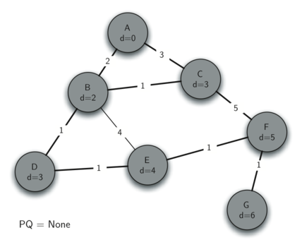
Finally, G can be explored as it is the only remaining vertex in the priority queue. With no edges that lead to vertices that are unconnected to the spanning tree, nothing can be updated when exploring G.

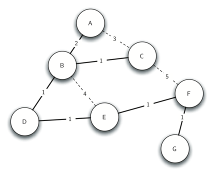
The output spanning tree is represented above overlaid on the graph, where solid lines represent the edges of the tree rooted at A that is uncovered by following the predecessor attribute from any given vertex. The dotted lines represent edges in the graph that do not make up a part of the output tree, as no predecessor link exists between the two vertices either side.