Source: 📖 Problem Solving with Algorithms and Data Structures using Python 8.20

---

Dijkstra's algorithm

Dijkstra's algorithm is used on graphs to find the shortest path between two vertices. It is somewhat similar to a breadth first search algorithm, so we must ensure that the Vertex class has certain attributes that allows it to operate (see Implementing breadth first search on a graph for implementation details). Using the BFS implementation as a starting point, we must now tweak it further by setting the self.distance attribute to the maximum possible value by default. We do this by importing the sys module and assigning self.distance to sys.maxint.

import sys
  

class Vertex:
  
	def __init__(self, key):
		self.key = key
		self.connected_to = {}
		self.distance = sys.maxint # change
		self.visited = False
		self.fully_searched = False
		self.predecessor = None
		self.discovered = None
		self.finished = None

	[...]

Next we need a priority queue, which we implement by tweaking a binary heap class:

class PriorityQueue(BinaryHeap):
  

	def __init__(self):
		self.heap = [(0, None)] # (priority, value)
		self.current_size = 0
	
	def percolate_up(self, i):
		while i // 2 > 0:
			if self.heap_list[i][0] < self.heap_list[i // 2][0]:
				self.heap_list[i], self.heap_list[i // 2] = self.heap_list[i // 2], self.heap_list[i]
			i = i // 2
	
	def percolate_down(self, i):
		while (i * 2) <= self.current_size:
			min_child_idx = self.min_child(i)
			if self.heap_list[i][0] > self.heap_list[min_child_idx][0]:
				self.heap_list[i], self.heap_list[min_child_idx] = self.heap_list[min_child_idx], self.heap_list[i]
			i = min_child_idx
	  
	def insert(self, priority, value):
		self.heap.append((priority, value))
		self.current_size += 1
		self.percolate_up(self.current_size)
	  
	def heapify(self, arr):
		i = len(arr) // 2
		self.current_size = len(arr)
		heap_list = [(vx.get_distance(), vx) for vx in arr]
		self.heap = [(0, None)] + heap_list[:]
		while i > 0:
			self.percolate_down(i)
			i -= 1
	  
	def extract_min(self):
		min_val = self.heap_list[1][0]
		self.heap_list[1] = self.heap_list[self.current_size]
		self.current_size -= 1
		self.heap_list.pop()
		self.percolate_down(1)
		return min_val
	  
	def change_priority(self, vx, new_priority):
		for i in range(1, self.current_size + 1):
			if self.heap_list[i][1] == vx:
				self.heap_list[i] = (new_priority, vx)
				self.percolate_up(i)
				self.percolate_down(i)
				break

The changes made allow the priority queue to implement a heap structure which accepts tuples with the format (priority, value), using priority as the key to order the heap with. The self.heap attribute establishes the (priority, value) format and the percolate methods index into the priority item within the tuple.

Finally, we can define Dijkstra's algorithm as follows:

def dijkstra(graph, start):
	pq = PriorityQueue()
	start.distance = 0
	pq.heapify([(vx.distance, vx) for vx in graph])
	while pq.size > 0:
		current_vx = pq.extract_min()
		for neighbour in current_vx.get_connections():
			new_distance = current_vx.distance + current_vx.get_weight(neighbour)
			if new_distance < neighbour.distance:
				neighbour.distance = new_distance
				neighbour.predecessor = current_vx
				pq.change_priority(neighbour, new_distance)

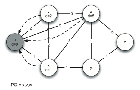
The dijkstra function takes two arguments – graph, a Graph object \(G\), and start, a Vertex object \(V\) where \(V \in G\). The first step the algorithm takes is to initiate an empty priority queue. Next, the distance attribute of the starting vertex is set to 0 (by default it is set to sys.maxint on Vertex initiation). Next we use a list comprehension to loop through all the vertices in graph and create (distance, vertex) tuples for our (priority, value) priority queue. The resulting list of tuples is turned into a priority queue using the heapify method.

Next we open a while loop that will stop when the priority queue is empty – it currently holds a (distance, vertex) tuple for each vertex in graph. Inside the loop, the first step is to extract the highest priority item in the priority queue – the item with the smallest distance, which is currently start as every other vertex's distance attribute is sys.maxint. We loop through each neighbouring vertex around start and read the weight of the edge from start to each neighbour. We calculate a new distance value for each neighbour to be the current vertex's distance plus the weight of the edge leading from the current vertex to the neighbouring vertex, then, if the new distance is less than the distance currently assigned to the neighbouring vertex, we overwrite its distance attribute with the lesser value and update its predecessor pointer to point to the current vertex, as a shorter path has been identified. Finally, with the distance attribute changed, the neighbour's priority in the priority queue also needs to be changed so we call change_priority on the neighbour vertex to update its distance value within the priority queue tuple that represents it.

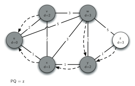
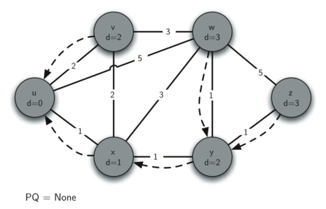
With one loop done, we go back to the start and the current_vx variable is updated to the next-closest vertex – that is, the vertex with the smallest distance value still in the priority queue. Since we've just finished the first loop over the start vertex, this pass will consider all neighbours of the closest neighbour to start. The loop will continue, each time choosing the next-closest vertex to start in the graph, until all vertices have been explored and their distance and predecessor attributes updated accordingly. When the loop is done, every vertex will be marked with its total distance to the start vertex and its shortest path back to start can be followed by tracing the predecessor attribute, vertex to vertex.

The following images illustrate the process. Edges are represented by solid arrows, with their weight values labeled. Dotted arrows represent predecessor pointers.